Perhaps the most important thing in finance is to control the risk or the exposition of your assets.
In fact, many portfolio managers would give up % of return to balance the risk of their assets. In this context, knowing how to measure risk is important, whether you are an individual investor who wants to maximize your gains or a portfolio manager who wants to beat a benchmark without risking your portfolio.
For this purpose, many metrics check the volatility of the asset through time and others do comparisons against a baseline to say how risky is the strategy. For the first case, we can mention Standard Deviation, as for the latter we have three important metrics: Sharpe Ratio, Beta, and Alpha.
For the metrics that we compare against a baseline, we usually define a “risk-free” percentage to compare against.
For instance, it’s good to compare the return investing in Treasury Securities, which is considered by many a secure investment, against your favorite asset. By doing this we’re checking if the return we’re obtaining in other assets is worth the risk (as we could do a “X” percent risk-free by investing in Treasury Securities alone).
Well, in this post we’ll explore these metrics, shedding light on how they work and why they matter.
Sharpe Ratio:
This metric measures the risk-adjusted return of an investment. It takes into account both the return and the risk (volatility) of the investment. A higher Sharpe Ratio indicates a better risk-adjusted performance. We calculate it by dividing the mean of the returns by the standard deviation of them.
Standard Deviation:
Standard Deviation is a measure of an investment’s volatility. It helps investors understand how much the returns deviate from the mean. A higher standard deviation suggests higher risk and potential for larger price swings.
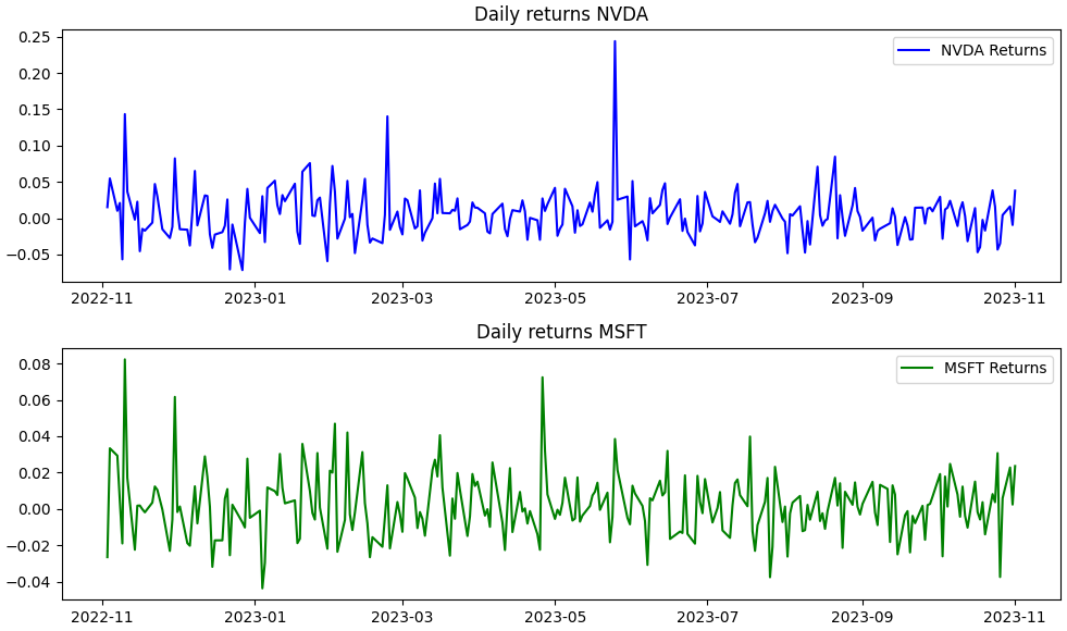
Now, let’s calculate both the Sharpe Ratio and Standard Deviation for NVDA and MSFT. This code below will also create a daily returns graph for both NVDA and MSFT
# importing libs
import yfinance as yf
import numpy as np
import matplotlib.pyplot as plt

# start and end
start_date = "2022-11-02"
end_date = "2023-11-02"

# download data
nvda = yf.download("NVDA", start=start_date, end=end_date)
msft = yf.download("MSFT", start=start_date, end=end_date)

# daily returns for both
nvda_returns = nvda['Adj Close'].pct_change().dropna()
msft_returns = msft['Adj Close'].pct_change().dropna()

# assuming 0% risk free rate (you can adjust it as needed)
risk_free_rate = 0

# sharpe ratio
nvda_sharpe_ratio = (nvda_returns.mean() - risk_free_rate) / nvda_returns.std()
msft_sharpe_ratio = (msft_returns.mean() - risk_free_rate) / msft_returns.std()

# (Standard Deviation)
nvda_std_deviation = nvda_returns.std()
msft_std_deviation = msft_returns.std()

# results
print("Sharpe Ratio NVDA:", nvda_sharpe_ratio)
print("Sharpe Ratio MSFT:", msft_sharpe_ratio)
print("Standard deviation NVDA:", nvda_std_deviation)
print("Standard deviation MSFT:", msft_std_deviation)

plt.figure(figsize=(10, 6))
plt.subplot(2, 1, 1)
plt.plot(nvda_returns, label="NVDA Returns", color='blue')
plt.title("Daily returns NVDA")
plt.legend()
plt.subplot(2, 1, 2)
plt.plot(msft_returns, label="MSFT Returns", color='green')
plt.title("Daily returns MSFT")
plt.legend()
plt.tight_layout()
Here are the results for this code
Sharpe Ratio NVDA: 0.15384885132315182
Sharpe Ratio MSFT: 0.11304841113168199
Standard deviation NVDA: 0.03390982717760015
Standard deviation MSFT: 0.01774081355502368
Also some graphs:
From these simple results, we can infer some new things
- Sharpe Ratio:
- Sharpe Ratio for NVDA: 0.1538Sharpe Ratio for MSFT: 0.1130
- Standard Deviation:
- Standard Deviation for NVDA: 0.0339
- Standard Deviation for MSFT: 0.0177
In summary, based on this information, NVDA had better risk-adjusted performance (higher Sharpe Ratio) over the past year but was also more volatile (higher Standard Deviation) compared to MSFT. We can notice by the graphs that NVDA had peaks over the year of up to 25% in a day (0.25 in the graph)
Notice by the code that we defined the risk-free rate as 0%, but if you define it as 2% for instance (0.02) you’ll notice the sharp value change. In this case, it’s better to allocate your capital to these risk-free assets, as the Sharpe ratio is negative:
Sharpe Ratio NVDA: -0.43595072563672094
Sharpe Ratio MSFT: -1.0142955821947708
Now some more complex metrics
Beta:
Beta measures the sensitivity of a stock’s returns to changes in the overall market. A Beta of 1 indicates that the stock tends to move in sync with the market, while a Beta greater than 1 suggests higher volatility, and less than 1 means lower volatility.
To calculate Beta for NVDA (NVIDIA Corporation) and MSFT (Microsoft Corporation) in Python, you can use the following pseudocode:
import yfinance as yf
import numpy as np

# Define the ticker symbols for NVDA and MSFT
nvda_ticker = "NVDA"
msft_ticker = "MSFT"

# Download historical data for NVDA and MSFT
nvda_data = yf.download(nvda_ticker, start="2022-11-02", end="2023-11-02")
msft_data = yf.download(msft_ticker, start="2022-11-02", end="2023-11-02")

# Calculate daily returns for NVDA and MSFT
nvda_returns = nvda_data['Adj Close'].pct_change().dropna()
msft_returns = msft_data['Adj Close'].pct_change().dropna()

# Download historical data for a market index (e.g., S&P 500) as a proxy for the market
market_data = yf.download("^GSPC", start="2022-11-02", end="2023-11-02")

# Calculate daily returns for the market index
market_returns = market_data['Adj Close'].pct_change().dropna()

# Calculate the Beta for NVDA and MSFT
cov_nvda_market = np.cov(nvda_returns, market_returns)[0][1]
var_market = np.var(market_returns)
beta_nvda = cov_nvda_market / var_market

cov_msft_market = np.cov(msft_returns, market_returns)[0][1]
beta_msft = cov_msft_market / var_market

# Print the Beta values for NVDA and MSFT
print("Beta for NVDA:", beta_nvda)
print("Beta for MSFT:", beta_msft)
Here are the results:
Beta for NVDA: 2.247229655892237
Beta for MSFT: 1.331273188102216
From this data, we can infer some new information
- Beta for NVDA (NVIDIA Corporation): A Beta of 2.24 suggests that NVDA is approximately 2.24 times more volatile (or has more systematic risk) compared to the overall market, which is often represented by the S&P 500. This means that NVDA’s returns tend to be more sensitive to market movements, both upward and downward.
- Beta for MSFT (Microsoft Corporation): A Beta of 1.33 indicates that MSFT is approximately 1.33 times as volatile as the overall market. MSFT’s returns are moderately sensitive to market movements.
In practical terms, a Beta greater than 1 indicates that the asset tends to move more significantly than the market, while a Beta less than 1 suggests that the asset is less volatile than the market.
If a portfolio manager is looking to create a strategy to simply beat the market with reduced risk, he can work with an allocation of X percent in NVDA and Y percent in MSFT, with buy and sell trades as needed. This way he can keep the beta near 1.
2.24*X + 1.33*Y = DESIRED_BETA
Notice X or Y may be negative if it’s a sell operation.
Also note that, just as we did the beta against the market, we can find the beta of one against the other, this would give us how much one varies from the other. Here is some code on how to do that:
import yfinance as yf
import numpy as np

nvda_ticker = "NVDA"
msft_ticker = "MSFT"

nvda_data = yf.download(nvda_ticker, start="2022-11-02", end="2023-11-02")
msft_data = yf.download(msft_ticker, start="2022-11-02", end="2023-11-02")

# Daily returns
nvda_returns = nvda_data['Adj Close'].pct_change().dropna()
msft_returns = msft_data['Adj Close'].pct_change().dropna()

# covariance of returns between NVDA and MSFT
cov_nvda_msft = np.cov(nvda_returns, msft_returns)[0][1]

# variance of MSFT returns
var_msft = np.var(msft_returns)

# calculating beta
beta_nvda_to_msft = cov_nvda_msft / var_msft

print("Beta NVDA to MSFT:", beta_nvda_to_msft)
Here’s the result
Beta NVDA to MSFT: 1.1699074740449837
So we can work with this data to reduce risk while keeping returns.
Finally, we have alpha:
Alpha:
Alpha represents the excess return on an investment relative to its Beta and the overall market return. A positive Alpha indicates outperformance, while a negative Alpha suggests underperformance.
To calculate Alpha, you need the stock’s actual returns, its expected returns based on Beta, and the actual market returns. The formula for Alpha is:
Alpha = Actual Returns – (Risk-Free Rate + Beta * (Market Returns – Risk-Free Rate))
Here’s the code calculating everything:
import yfinance as yf
import numpy as np

# Define ticker symbols for NVDA, MSFT, and the S&P 500 index (e.g., SPY ETF)
nvda_ticker = "NVDA"
msft_ticker = "MSFT"
sp500_ticker = "SPY"

# Download historical data for NVDA, MSFT, and the S&P 500 index
nvda_data = yf.download(nvda_ticker, start="2022-11-02", end="2023-11-02")
msft_data = yf.download(msft_ticker, start="2022-11-02", end="2023-11-02")
sp500_data = yf.download(sp500_ticker, start="2022-11-02", end="2023-11-02")

# Calculate daily returns for NVDA, MSFT, and the S&P 500 index
nvda_returns = nvda_data['Adj Close'].pct_change().dropna()
msft_returns = msft_data['Adj Close'].pct_change().dropna()
sp500_returns = sp500_data['Adj Close'].pct_change().dropna()

# Calculate beta for NVDA
covariance_nvda = np.cov(nvda_returns, sp500_returns)
beta_nvda = covariance_nvda[0, 1] / np.var(sp500_returns)

# Calculate beta for MSFT
covariance_msft = np.cov(msft_returns, sp500_returns)
beta_msft = covariance_msft[0, 1] / np.var(sp500_returns)

# Calculate alpha for NVDA
alpha_nvda = nvda_returns.mean() - (0 + beta_nvda * (sp500_returns.mean() - 0))

# Calculate alpha for MSFT
alpha_msft = msft_returns.mean() - (0 + beta_msft * (sp500_returns.mean() - 0))

# Print the values of betas and alphas
print("Beta for NVDA:", beta_nvda)
print("Alpha for NVDA:", alpha_nvda)
print("Beta for MSFT:", beta_msft)
print("Alpha for MSFT:", alpha_msft)
Results from the code:
Beta for NVDA: 2.247229655892237
Alpha for NVDA: 0.003892889146694762
Beta for MSFT: 1.331273188102216
Alpha for MSFT: 0.0012211661673088427
For NVDA:
- The alpha of 0.0039 is positive, which means that NVDA has outperformed the expected return, given its level of risk (beta) and the assumed risk-free rate (0). In other words, NVDA has generated a return that is approximately 0.39% higher than what would be expected based on its exposure to market risk. A positive alpha suggests that NVDA has delivered positive excess returns compared to the market.
For MSFT:
- The alpha of 0.0012 is also positive, which means that MSFT has outperformed the expected return, given its level of risk (beta) and the assumed risk-free rate (0). In this case, MSFT has generated a return that is approximately 0.12% higher than what would be expected based on its exposure to market risk. Similar to NVDA, a positive alpha for MSFT suggests that it has delivered positive excess returns compared to the market.
In summary, both NVDA and MSFT have positive alphas, indicating that they have provided returns exceeding what would be expected based on their risk profiles and the assumption of a risk-free rate of 0. Of course, the risk-free tax we can achieve is a bit higher than 0% so you need to make sure the volatility is worth the risk.
That’s it for this post!
Hope you learned something new about how to measure the risk of your assets and compare it against the market!
Feel free to comment about it below and ask for specific posts!